ABSTRACT
This report presents the numerical analysis of a Tesla valve to validate its diodicity using CFD
simulations. Steady-state and transient flows were analyzed using simpleFoam and pimpleFoam
solvers, respectively. Pressure drop is evaluated for forward and reverse flow. The results demonstrate
clear asymmetry in flow resistance, confirming the valve’s diode-like performance. The simulation
results were validated against previously published experimental data from Zhao et al. (2024). Grid
independence, solver comparison, and validation are also included to ensure the reliability of the
simulation results.
INTRODUCTION:
The Tesla valve is a passive device with no moving parts that allows fluid to flow more easily in one
direction while restricting flow in the opposite direction. Its unique geometry creates asymmetric flow
resistance, which makes it useful in applications such as microfluidics, cooling systems, and other
passive flow-control systems. In this study, CFD simulations were employed to evaluate the diodicity of
a Tesla valve by analyzing pressure drops. Diodicity (𝐷𝑖) is the ratio of reverse to forward pressure
drop. If 𝐷𝑖>1, the valve is more effective, meaning it offers more resistance to reverse flow than to
forward flow. The simulations were conducted using simpleFoam for steady-state and pimpleFoam for
transient flow, capturing both steady and time-dependent behaviors. A grid-independent study is
performed to ensure the accuracy of numerical results. The objective of this work is to numerically
validate the diode-like behavior of the Tesla valve.
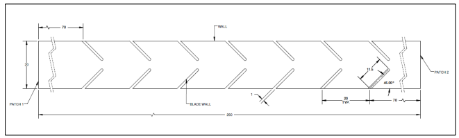
BOUNDARY CONDITIONS:
I. Flow Direction
Two simulations were performed to evaluate the Diodicity of the Tesla valve. For forward flow, Patch
1 is assigned as the inlet and Patch 2 as the outlet, and vice versa for reverse flow.
II. Fluid Properties
Fluid : Water
Temperature, T : 20 °C
Density, ρ : 998.29 kg/m3
Dynamic viscosity, µ : 0.001002 Pa-s
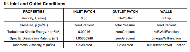
Velocity:
A fixedValue boundary condition of 0.35 m/s is applied at the inlet to prescribe the inflow. At the outlet,
an inletOutlet boundary condition is used, which enforces a zero-velocity condition for any potential
backflow while allowing a zeroGradient condition when the flow exits the domain. At all solid walls, a
no-slip boundary condition is imposed, such that the fluid velocity is zero at the wall surface.
Pressure:
A zeroGradient boundary condition is applied at the inlet, allowing the pressure to adjust naturally
according to the flow field. At the outlet, a totalPressure boundary condition with a reference value of
zero is applied, ensuring that the total pressure is fixed at the exit while allowing the static pressure to
adjust according to the local velocity. At the solid walls, a zeroGradient condition is applied, enforcing
no normal pressure variation at the wall.
Turbulent Kinetic Energy (k):
A fixed value of 0.00046 m2
/s2
is given to define the incoming turbulence level. At the outlet, a
zeroGradient condition is applied, allowing the turbulence to leave the domain naturally without
enforcing the fixed value. The kqRWallFunction is applied to model how turbulence behaves very close
to the wall, where turbulence naturally reduces due to viscosity.
Specific Dissipation Rate (ω):
A fixed value of 1.95655948 s-1
is specified at the inlet based on the inlet turbulence properties. At the
outlet, a zeroGradient condition allows ω to exit the domain smoothly. At the walls, the
omegaWallFunction is applied to represent near-wall turbulence dissipation.
Turbulent Kinematic Viscosity (νₜ):
The turbulent viscosity is calculated internally by the solver at both the inlet and outlet form the
turbulence variables k and ω. At the walls, a nutUBlendedWallFunction is applied, that automatically
blends low-Re (viscous sublayer) and high-Re (inertial/log law) predictions using a smooth, binomial
blending method, offering a single condition for varying y+ values.
SOLVER SETUP
Time Schemes:
Both steady-state and unsteady (transient) simulations were performed. For the steady-state analysis,
a steadyState time discretization scheme was used, assuming time-independent flow conditions. For
the unsteady analysis, a first-order Euler time discretization scheme was used, assuming timedependent flow conditions.
Gradient Schemes:
All spatial gradients are computed using the Gauss linear scheme. The Gauss option represents the
standard finite-volume discretization based on Gaussian integration, which requires interpolation of
variables from cell centers to face centers. The linear interpolation corresponds to central differencing
and provides second-order spatial accuracy.
Divergence Schemes:
I. Velocity convection (div(phi, U)): The Gauss linearUpwind scheme with velocity gradient
reconstruction is used. This is a second-order, upwind-biased scheme that improves numerical stability
in turbulent flows while maintaining reasonable accuracy.
II. Turbulence equations (k, ω): A bounded Gauss limitedLinear scheme is applied to the convection
of turbulence variables. This limits numerical overshoots and ensures physically realistic, stable
solutions for turbulence quantities.
III. Viscous stress term: The diffusive term involving the effective viscosity is discretized using a Gauss
linear scheme, providing accurate representation of viscous effects.
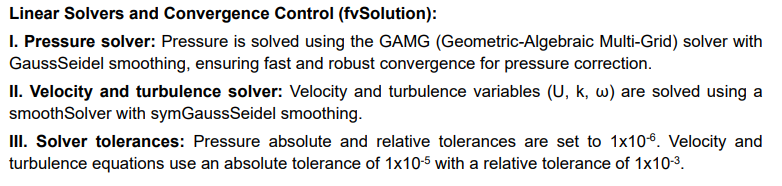
SIMPLE Algorithm:
The SIMPLE algorithm is used for pressure-velocity coupling in the steady-state simulations. No nonorthogonal correctors are applied (nNonOrthogonalCorrectors = 0) since the mesh non-orthogonality is
within acceptable limits. Convergence is monitored using residual control, where the solution is
considered when the residuals of pressure, velocity, and turbulence quantities fall below 1×10
-5
.
PIMPLE Algorithm:
The PIMPLE algorithm is used for unsteady simulations to couple pressure and velocity. A momentum
predictor is enabled, and multiple pressure-velocity correction loops are applied within each time step
to improve stability and convergence. No non-orthogonal correctors are used since the mesh quality is
within acceptable limits.
Relaxation Factor:
Under-relaxation factors of 0.7 are applied to the velocity equation and all remaining governing
equations to enhance numerical stability during the iterative solution process. This controlled relaxation
prevents abrupt changes in the solution variables between iterations and supports the solution
converge smoothly and remain numerically stable.
GRID INDEPENDENCE STUDY
A grid independence study was conducted to ensure that the numerical solution obtained using
simpleFoam is not significantly influenced by mesh size. The baseline grid consists of 264 x 14 x 24
cells, and two additional meshes were generated by scaling the base mesh by 0.8x (coarse) and 1.2x
(fine).
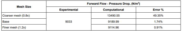
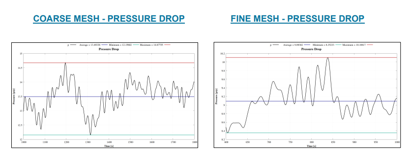
The coarse mesh produced a significant deviation from experimental results, indicating insufficient
resolution to capture the flow physics reliably. The base mesh and the refined mesh both showed less
errors of 1.74% and 1% respectively. Since the difference between the base mesh and refined mesh is
minimal (~ less than 1%), the base grid (264 x 14 x 24) is sufficiently fine for accurate predictions. The
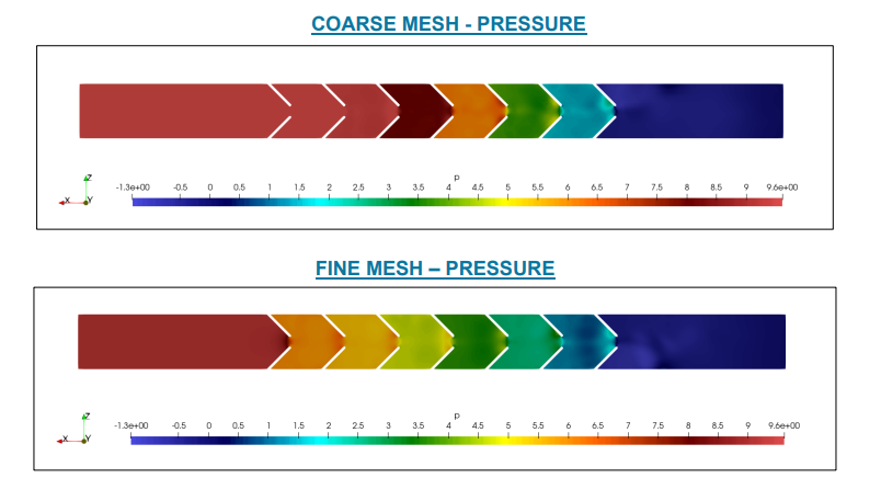
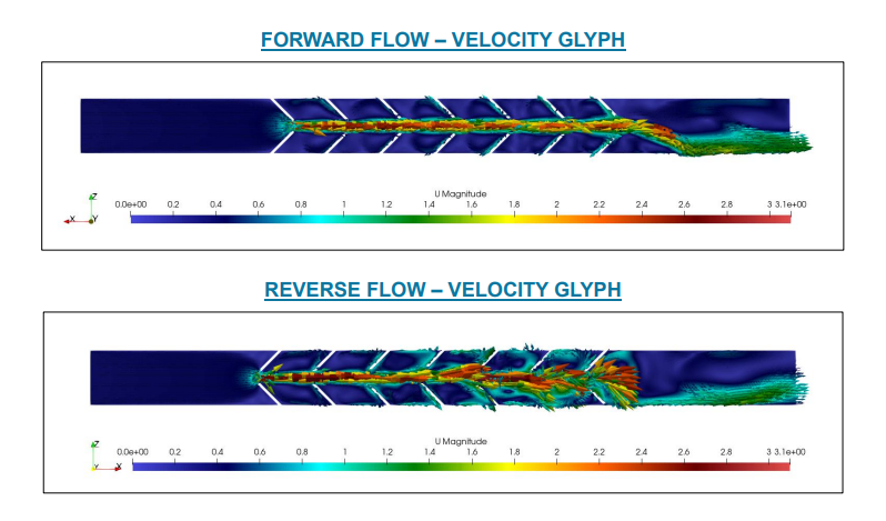
base mesh is selected for all subsequent simulations as it offers a good balance between computational
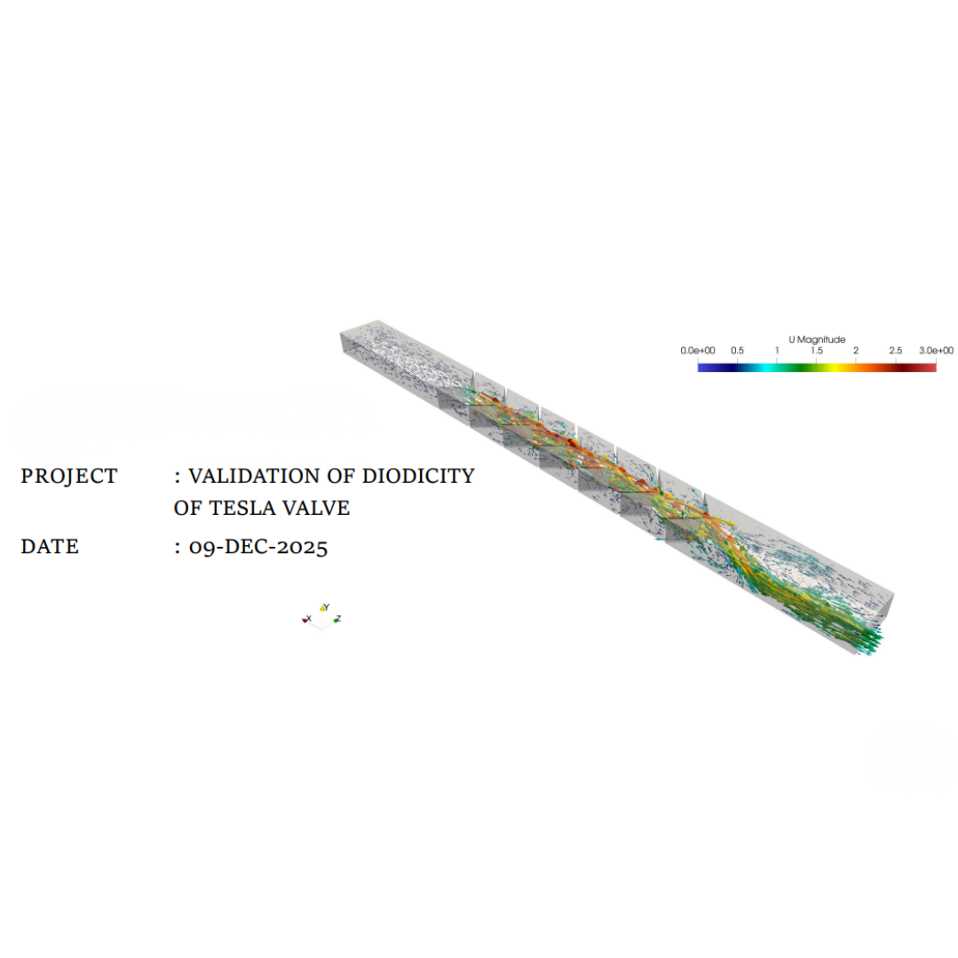
cost and accuracy. The corresponding pressure-drop plots and velocity-field glyphs are provided below.
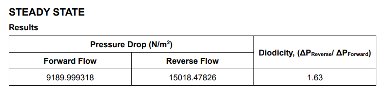
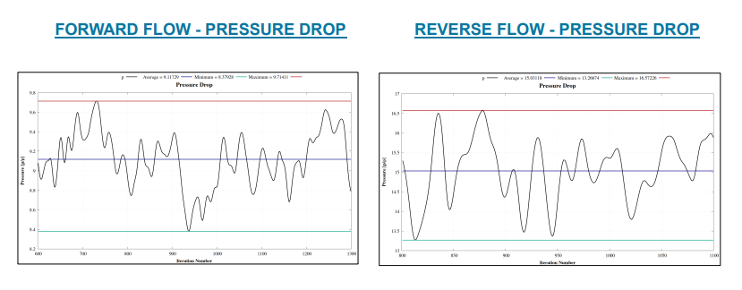
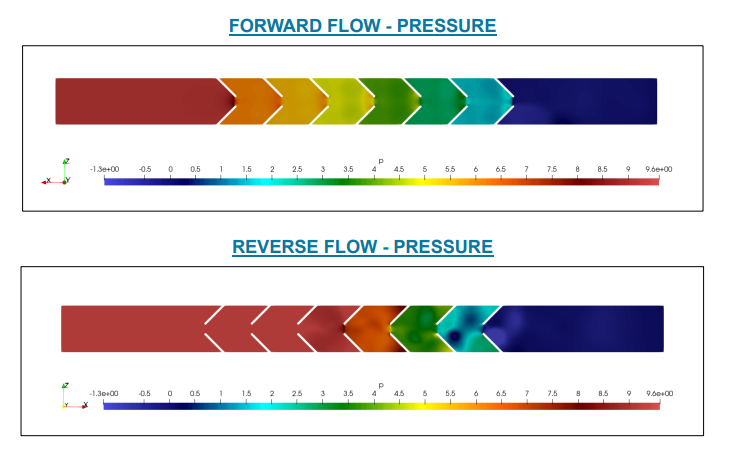
The forward-flow pressure-drop obtained from the simulation is 9189.99 N/m2
, while the reverse-flow
pressure-drop is 15018.48 N/m2
. The resulting diodicity, defined as the ratio of reverse to forward
pressure drop, is 1.63, indicating higher resistance in the reverse direction. All numerical results were
generated using a steady-state simulation with the simpleFoam solver and the k-ω SST turbulence
model. The corresponding pressure-drop distributions and velocity-field glyphs are provided below to
support the validation of the numerical model.
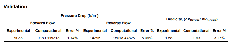
The validation of the steady state simpleFoam solver was carried out by comparing the computed
pressure drops and diodicity with the experimental data. The forward-flow pressure drop shows an error
of 1.74%, while the reverse-flow pressure-drop exhibits an error of 5.06%. The predicted diodicity (1.63)
differs from the experimental value (1.58) by 3.27%, demonstrating good agreement and confirming
the reliability of the steady-state CFD model
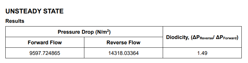
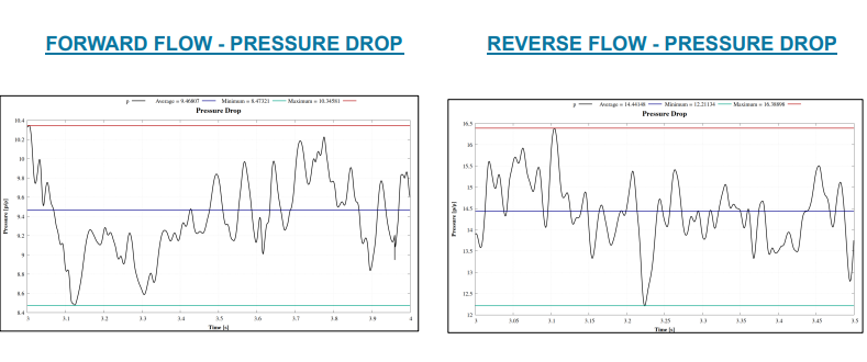
The forward-flow pressure-drop obtained from the simulation is 9597.72 N/m2
, while the reverse-flow
pressure-drop is 14318.03 N/m2
. The resulting diodicity, defined as the ratio of reverse to forward
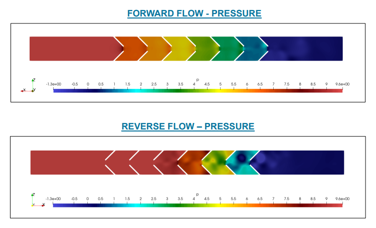
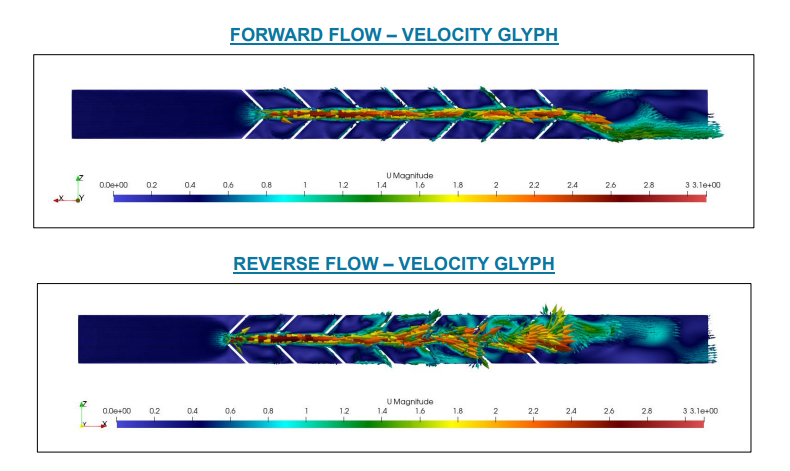
pressure drop, is 1.49, indicating higher resistance in the reverse direction. All numerical results were
generated using a unsteady-state simulation with the pimpleFoam solver and the k-ω SST turbulence
model. The corresponding pressure-drop distributions and velocity-field glyphs are provided below to
support the validation of the numerical model.
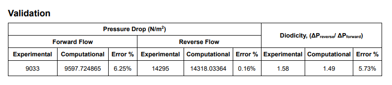
The validation of the unsteady pimpleFoam solver was performed by comparing the computed pressure
drops and diodicity with experimental data. The forward-flow pressure drop shows an error of 6.25%,
while the reverse-flow pressure-drop exhibits a very small error of 0.16%. The predicted diodicity (1.49)
differs from the experimental value (1.58) by 5.73%, indicating good agreement and acceptable
accuracy of the unsteady CFD model.
STEADY-STATE vs UNSTEADY-STATE SOLVER PERFORMANCE ANALYSIS
A comparison of the steady-state (simpleFoam) and unsteady (pimpleFoam) simulations shows that
both models capture the experimental pressure drop behaviour with less than 10% error. The steadystate simulation gives a forward-flow pressure-drop error of 1.74% and a reverse flow error of 5.06%,
resulting in a diodicity error of 3.27%. In contrast, the unsteady simulation gives a forward-flow
pressure-drop error of 6.25% and a reverse flow error of 0.16%, resulting in a diodicity error of 5.73%.
Based on these results, the steady-state solver with the k-ω SST turbulence model is sufficiently
accurate and provides reliable predictions of the pressure drop and diodicity of the Tesla valve, while
requiring low computational cost compared to the transient solver.
CONCLUSION
This study numerically evaluated the diodicity of a Tesla valve using CFD simulations in OpenFOAM,
employing both steady-state and transient solvers. Pressure drops in forward and reverse directions
were analysed, and both solvers successfully captured the asymmetric flow resistance characteristic
of the valve. The steady-state solver produced highly accurate predictions with minimal computational
cost, while the transient solver provided similar accuracy with significantly greater computational effort.
The grid independence study confirmed that the chosen mesh resolution was sufficient to capture the
complex flow structures that contribute to the valve’s asymmetric resistance. Validation against
experimental data from Zhao et al. (2024) demonstrated strong agreement, with diodicity errors within
3–6%, confirming the reliability of the CFD methodology. Overall, the results verify that OpenFOAM can
accurately simulate the diode-like behaviour of Tesla valve. The validated model may be applied in
future work to optimize the Tesla valve geometry for improved diodicity.
BIBLIOGRAPHY
Y.-J. Zhao, J.-B. Tong, Y.-L. Zhang, X.-W. Xu, L.-H. Tong. (2024). Hydraulic loss experiment of straightthrough Tesla valve in forward and reverse directions. Processes, 12(7), 11418266.
(https://pmc.ncbi.nlm.nih.gov/articles/PMC11418266/)